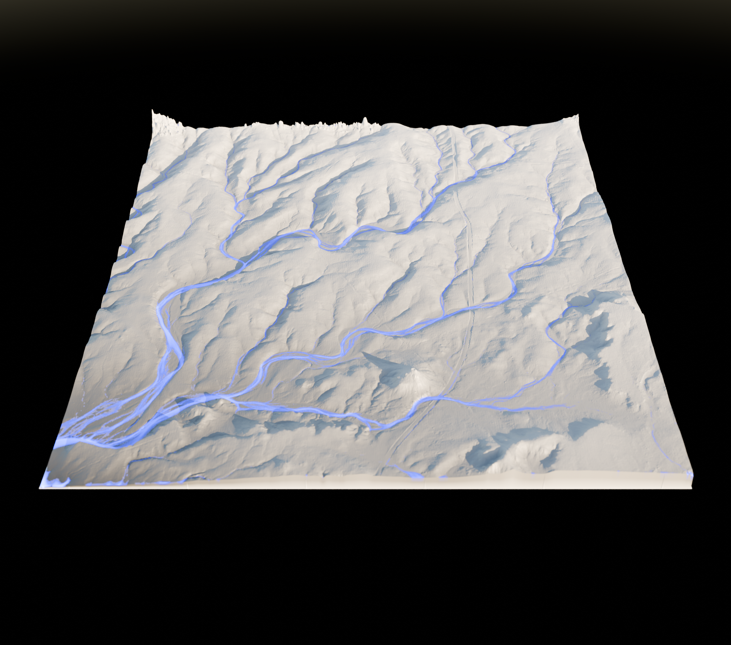
💧Getting Started on Graphflood
Table of Contents
##
Quick Start
While I am still constructing the documentation I provide on this page quick ways to use graphflood.
You need to have:
- 2D topography (DEM file, premade function, anything that provide a 2D regular grid of elevation)
- Precipitation rates (scalar, 2D array)
- Manning coefficient (scalar, 2D array) -> 0.033 is a commonly accepted value in rivers
- [if needed] 2D Boundary conditions
- [If not done yet]
scabbardinstalled
You need to now
- Every backend has different pros and cons and may produce slightly different results.
gpubackend is a lot faster, but you need a GPU with enough memorygraphfloodis iterative, you need to decide on a convergence criterion (easy solution: run until the flow depth stabilises)- Higher
dt= faster convergence, but more instabilities. I am working on adding automaticdtand convergence detection.
**
#
Simple Setup
DEM has no NoData, flow can out from every edges of the model
Default Boundary Conditions
import matplotlib.pyplot as plt
import numpy as np
import taichi as ti
import scabbard as scb


# Loading the DEM
grid = scb.io.load_raster('dem.tif')


# Change this variable to change the backend:

## GPU backend with taichi
### (if you have a MAC this remains untested but theoretically works)
### (If you are on Linux/Windows WITHOUT Nvidia GPU, you need to install the vulkan SDK/drivers -> https://vulkan.lunarg.com/)
# backend = 'gpu'
# ti.init('gpu')
## CPU backend with DAGGER (OG graphflood - both options work)
# backend = 'cpu'
# backend = 'dagger'

## CPU libTopoToolbox backend
backend = 'ttb'

# running Graphflood dor 1000 iterations
results = scb.graphflood.std_run(
    grid, # Sting or grid so far
    P = 1e-4, # precipitations, 2D numpy array or scalar
    BCs = None, # Boundary codes
    N_dt = 500,
    backend = backend,
    dt = 1e-2,
    init_hw = None) # init_hw can be a 2D array of DEM dimension with pre-existing flow depth. For example if you want to continue a run

fig,ax = scb.visu.hillshaded_basemap(grid)


hw = results['h'].Z.copy() # if ttb is used, results arrays are topotoolbox GridObj
hw[hw<0.01] = np.nan
im = ax.imshow(hw, cmap = 'Blues', vmax = 3., extent = grid.geo.extent, alpha = 0.75)
plt.colorbar(im, label = 'Flow Depth (m)')
plt.show()
#
Isolating sub-section of a DEM
DEM has NoData, or for any other reason will not consider some nodes (e.g. bellow sea level, only the main watershed, ...)
Use of automatic functions to set up the Boundary Conditions
import matplotlib.pyplot as plt
import numpy as np
import taichi as ti
import scabbard as scb


# Loading the DEM
grid = scb.io.load_raster('dem.tif')

# Isolating the main drainage basin
## this function returns a mask of 0,1 showing the main watershed
mask = scb.flow.mask_main_basin(grid, MFD = False)
## You could also, alternatively, mask seas in case you wanna remove all the data below a certain values
# mask = mask_seas(grid, sea_level = 0.)

## Encode the mask into boundary conditions
BCs = scb.flow.mask_to_BCs(grid,mask)

# Change this variable to change the backend:

## GPU backend with taichi
### (if you have a MAC this remains untested but theoretically works)
### (If you are on Linux/Windows WITHOUT Nvidia GPU, you need to install the vulkan SDK/drivers -> https://vulkan.lunarg.com/)
backend = 'gpu'
## CPU backend with DAGGER (OG graphflood - both options work)
# backend = 'cpu'
# backend = 'dagger'

## CPU libTopoToolbox backend
# backend = 'ttb'

# running Graphflood dor 1000 iterations
results = scb.graphflood.std_run(
    grid, # Sting or grid so far
    P = 1e-4, # precipitations, numpy array or scalar
    BCs = BCs, # Boundary codes
    N_dt = 5000,
    backend = backend,
    dt = 1e-2,
    init_hw = None)

fig,ax = scb.visu.hillshaded_basemap(grid)


hw = results['h'].copy()
hw[hw<0.01] = np.nan
im = ax.imshow(hw, cmap = 'Blues', vmax = 3., extent = grid.geo.extent, alpha = 0.75)
plt.colorbar(im, label = 'Flow Depth (m)')
plt.show()
#
Reach Mode: modelling a local trunk with entry fluxes
Coming soon: how to finely manage boundary conditions in a case where I want to input flow on the left edge of my DEM, and force it to only output at the right edge
