CHONK

B. Gailleton, L. Malatesta, G. Cordonnier, J. Braun, B. Bovy

This page gets updated regularly with info about CHONK and will point to the new model documentation soon

What is CHONK?

CHONK is a numerical framework for Landscape Evolution Modelling (LEM) currently in development. A numerical framework provides tools and numerical structure to design, run and analyse model - for example LANDLAB is a mature LEM framework. CHONK mixes classic LEM principles and algorithms - e.g. graph theory controlling cell topology - with cellular automata data structure. The latter is the novelty: every aspect of the simulation is expressed in a cell referential. To build a cell, the user only needs to define properties (e.g. elevation, drainage area, erosion, tracker) and functions (e.g. fluvial erosion, water transport, diffusion) describing how the properties interact within the cell and with the neighbourhood.

This prototype is available here, but is not generic and hard to custom with new laws. A second version is currently being developed with a flexible python interface to build the model structure and run/analyse the simulations. It provides a lot of flexibility to design an abstract model structure which is then compiled with cython into a c++ core engine.

What can CHONK do?

The cellular-automata structure and the intended flexibility add an inevitable small computational overhead. However, it provides a crucial advantage: because all the functions are processed for a cell before moving to the next, the final state of properties is known.

Endorehism, internally drained basins and local minima

At any point in the simulation, we can know the final state of fluxes in the cell. If water and sediments are part of the cell we can use them to fill local minima with a finite amount of water and sediment to know what will be transferred downstream. This level of detail is not necessary for all studies and we provide different methods to deal with local minima. Using Cordonnier et al. 2019, we provide an implicit lake solver. It reroutes flow from the bottom of a depression to its outlet either directly, or via carving/filling algorithms. This methods intends to ensure flow continuity (i.e. water does not simply stops at the local minima) but does not consider explicitly the lake topography. We developed another method, inspired from Barnes et al., 2020 which builds local binary trees of depression systems to being able to know the volume each single depression or depression system can store. It allows us to process lake as fully separated domains with dedicated process law, including potentially evaporation. Mixed with graph theory, we can calculate a topological order and process cells from upstream to downstream. You can find bellow a comparative study in a case where using different solvers makes significant differences (Note that it does not mean it is crucial for ALL case studies).

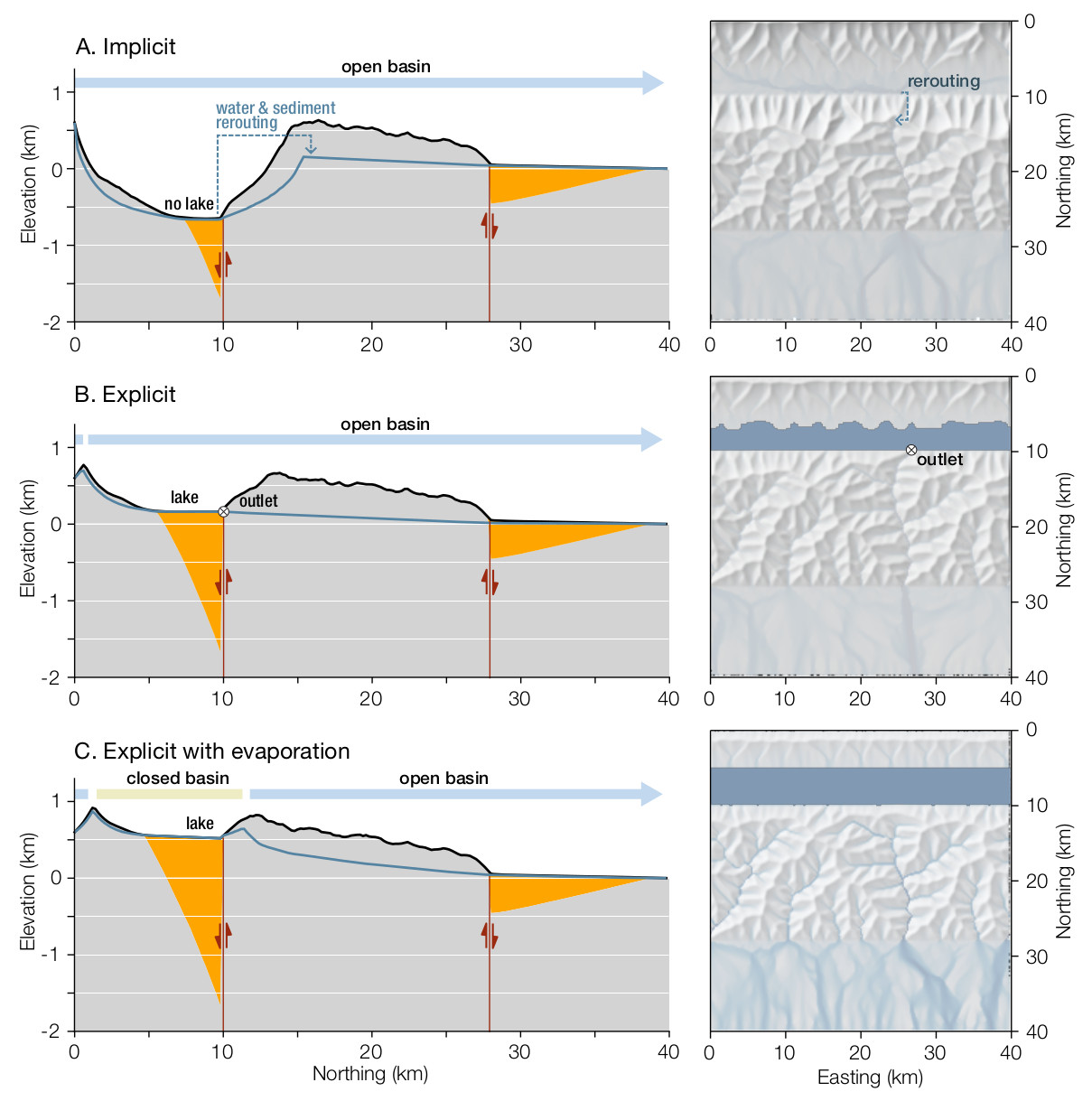Different results for different lake solver on a landscapes with an internal normal fault.

Tracking fluxes and quantities

As all the process laws affecting fluxes and quantities are processed at once, it makes the tracking of elements easier. Theoretically these could be anything geochemical, provenance, timing, … . This tracking can also be done in the stratigraphy as the model allows the stacking of information in the stratigraphy. We tested this tracking capabilities by simply adding a “granitoid-like” patch of rock and investigating where does it go.

Detailed tracking of the provenance of sediments coming the granitoids, including recycled

Internal dynamic feedbacks

Again, because we always know what is inside the cell, we can express feedback between the different properties. For example, as a simple exercise, we can roughly approximate a “tool effect” by modulating fluvial erosion function of the rock type of the mobile sediments. With a similar scenario than above, we consider our “granitoid” as a harder rock than the surrounding bedrock. When the mobile sediment flux contains granitoids sediment and erode less resistant basement, we increase fluvial erosivity, and we decrease it in the opposite scenario. We then observed the final river long profile and compared it to a vanilla scenario.

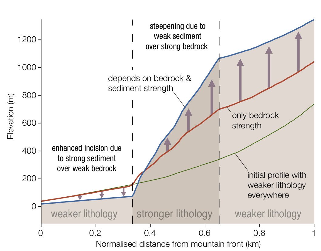Illustration of non-local effect linked to the tool effect.